Demystifying Logistic Regression
For our hackathon this week, I, along with several co-workers, decided to re-implement Vowpal Wabbit (aka "VW") in Go as a chance to learn more about how logistic regression, a common machine learning approach, works, and to gain some practical programming experience with Go.
Though our hackathon project focused on learning Go, in this post I want to spotlight logistic regression, which is far simpler in practice than I had previously thought. I'll use a very simple (perhaps simplistic?) implementation in pure Python to explain how to train and use a logistic regression model.
Predicting True or False
Logistic regression is a statistical learning technique useful for predicting the probability of a binary outcome -- true or false. As we've previously written, we use logistic regression with VW to predict the likelihood of a user clicking on a particular ad in a particular context, a true or false outcome.
Logistic regression, like many machine learning systems, learns from a "training set" of previous events, and tries to build predictions for new events it hasn't seen before. For instance, we train our click prediction model using several weeks of ad views (impressions) and ad clicks, and then use that to make predictions about new events to determine how likely the user is to click on an impression.
Each data point in the training set is further broken down into "features," attributes of the event that we want the model to learn from. For online advertising, common features include the size of the ad, the site on which the ad is being shown, the location of the user viewing the ad, and so on.
Logistic regression, or more accurately, Stochastic Gradient Descent, the algorithm that trains a logistic regression model, computes a weight to go along with each feature. The prediction is the sum of the products of each feature's value and each feature's weight, passed through the logistic function to "squash" the answer into a number in the range [0.0, 1.0].
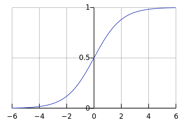 The standard logistic function. Public Domain image from
Wikipedia by
Qef.
The standard logistic function. Public Domain image from
Wikipedia by
Qef.
Applying a logistic regression model is therefore relatively easy, it's a simple loop to write. What surprised me most during the hackathon project is that training a logistic regression model, coming up with the values for the weights we multiply by the features, is also surprisingly concise and straightforward.
An Example
Let's consider a click data set. Each row in the table is an event we've (hypothetically) recorded, either an impression which did not get a click, or an impression plus click, along with a series of attributes about the event that we'll use to build our regression model.
| Size | Site | Browser | State | EventType |
|---|---|---|---|---|
| 160x600 | wunderground.com | IE | AZ | impression |
| 160x600 | ebay.com | IE | IA | click |
| 728x90 | msn.com | IE | MS | impression |
| 160x600 | ebay.com | Chrome | FL | impression |
| 728x90 | popularscience.tv | Chrome | CA | impression |
| 320x50 | weather.com | Chrome | NB | impression |
| 300x250 | latimes.com | Firefox | CA | impression |
| 728x90 | popularscience.tv | IE | OR | impression |
| 300x250 | msn.com | Chrome | MI | impression |
| 728x90 | dictionary.com | Chrome | NY | impression |
| 300x250 | ebay.com | Safari | OH | impression |
| 320x50 | msn.com | Chrome | FL | click |
| 728x90 | dictionary.com | Chrome | NJ | impression |
| 728x90 | urbanspoon.com | Firefox | OR | impression |
| 728x90 | msn.com | Chrome | FL | impression |
| 728x90 | latimes.com | Chrome | AZ | impression |
| 728x90 | realtor.com | Chrome | CA | impression |
| 728x90 | deviantart.com | Chrome | DC | impression |
| 728x90 | weather.com | IE | OH | click |
| 728x90 | msn.com | IE | AR | impression |
| 728x90 | msn.com | IE | MN | impression |
| 300x250 | wunderground.com | Chrome | MI | impression |
| 300x250 | dictionary.com | IE | OK | impression |
| 300x250 | popularscience.tv | Chrome | IN | impression |
| 300x250 | dictionary.com | Chrome | MA | impression |
| 300x250 | weather.com | Chrome | VT | impression |
| 320x50 | ebay.com | Chrome | OH | click |
| 300x600 | popularscience.tv | IE | NJ | impression |
| 728x90 | weather.com | IE | WA | impression |
| 300x250 | weather.com | IE | MO | impression |
These 30 data points will form our training data set. The model will learn from these examples what impact the attributes -- size, site, browser, and US state -- have on the likelihood of the user clicking on an ad that we show them.
In reality, to build a good predictive model you need many more events than the 30 that I am showing here -- we use tens of millions in our production modeling pipelines in order to get good performance and coverage of the variety of values that we see in practice.
To convert this data set to work with logistic regression, which computes a binary outcome, we'll treat each click as a target value of 1.0, also known as a "positive" event, and each impression as 0.0, or a "negative" event.
We also need to account for the fact that each of our features is a string, but logistic regression needs features that have values that it can multiply by its weight to compute the sum-of-products. Our features don't have numeric values, just some set of possibilities that each attribute can take on. For instance, the size attribute is one of three ad sizes we work with, 300x250, 728x90, or 160x600. Features that can take on some set of discrete values are called "categorical" features.
We could assign a numeric value to each of the possibilities, for instance use the value 1 when the size is 300x250, 2 when the size is 728x90, and 3 when the size is 160x600. This would work mechanically, but won't produce the outcome that we want. Since the weight of the feature "size" is multiplied by the value of the feature in each event, this would mean that we've decided, arbitrarily, that 160x600 is three times more "clicky" than 300x250, which the data set may not bear out. Moreover, for some attributes, like site, we have many many possible values, and determining what numeric value to assign to each of the possiblities is tedious, and will further amplify the problem as described here.
The proper solution to this problem is as effective as it is elegant: rather than having 1 feature, "site" with values like "ebay.com" or "msn.com", we create a much larger set of features, one for each site that we have seen in our training or evaluation data set. For a given training data example, if the "site" column has value "msn.com", we say that the feature "site:msn.com" has value 1, and that all other features in the "site:..." family have value 0. Essentially, we pivot the data by all the values of each categorical feature. Of course, the total number of features in our training set becomes very large, but, as we will see, SGD can accomodate this gracefully.
Stochastic Gradient Descent In Action
At the start of the hackathon, we wrote some very simple Python code to serve as a reference for how logistic regression should work. Python reads almost like pseudocode, so thats what we'll show here, too.
We decided to model examples as Python dictionaries, with a top-level field indicating the actual outcome (1.0 for clicks, 0.0 for impressions), and a nested dictionary of features. Here's what one looks like:
{
    "actual": 1.0,
    "features": {
        "site": "ebay.com",
        "size": "160x600",
        "browser": "IE",
        "state": "IA",
    }
}
Given an example and a dictionary of weights, we can predict the outcome
straighforwardly:
def predict(weights, example):
    score = 0.0
    for feature in extract_features(example):
        score += weights.get(feature, 0.0)
    score += weights.get("bias", 0.0)
    return 1.0 / (1 + math.exp(-score))
We initialize the score to 0, then for each feature in the example, we get the weight from the dictionary. If the weight doesn't exist (because the model hasn't been trained on any examples containing this feature), then we assume 0 as the weight, which leaves the score as-is.
Additionally, we add in a "bias" weight, which you can think of as a feature that every example has. The "bias" weight helps SGD correct for an overall skew in our training data set one way or another. It's possible to leave this out, but it's generally helpful to keep it.
The expression at the end of this function is the logistic function, as we saw
above, which squashes the result into the range 0 to 1. We do this because we
are trying to predict a binary outcome, so we want our prediction to be
strictly between these two boundary values. If you do the math, you'll see
that for an empty model -- one with nothing in the weights dictionary -- we
will predict 0.5 for any input example.
Generating the features we use in SGD from our example is similarly straightforward:
def extract_features(example):
    return example["features"].iteritems()
Since our features are categorical, we can take advantage of Python's
dictionary to generate (key, value) pairs as the actual features. Though all
our examples have values for each of the four attributes we're considering,
they each have different values -- thus the tuples generated by
extract_features will be different for each example. This is our conversion
from attributes with a set of possible values, to features which carry the
implicit value 1.
Finally, we have enough code in place to see how stochastic gradient descent training actually works:
def train_on(examples, learning_rate=0.1):
    weights = {}
    for example in examples:
        prediction = predict(weights, example)
        actual = example["actual"]
        gradient = (actual - prediction)

        for feature in extract_features(example):
            current_weight = weights.get(feature, 0.0)
            weights[feature] = current_weight + learning_rate * gradient

        current_weight = weights.get("bias", 0.0)
        weights["bias"] = current_weight + learning_rate * gradient

    return weights
For each example in the training set, we first compute the prediction, and,
along with the actual outcome, we compute the gradient. The gradient is a
number between -1 and 1, and helps us adjust the weight for each feature, as
we'll see in a moment.
Next, for each feature in the example, we update the weight for that feature
by adding or subtracting a small amount from the current weight, the
learning_rate. Here we can now see how the gradient works in action.
Consider the case of a positive example (a click). The actual value will be
1.0, so if our prediction is high (close to 1.0), we'll adjust the weights up
by a small amount; if the prediction is low, the gradient will be large, and
we'll adjust the weights up by a correspondingly large amount. On the other
hand, consider when the actual outcome is 0.0 for a negative event. If the
prediction is high, the gradient will be close to -1, so we'll lower the
weight by a relatively large amount; if the prediction is close to 0, we'll
lower the weight by a relatively small amount.
For the first example, or more generally, the first time a given feature is seen, the feature weight is 0. But, since each example has a different set of features, over time the weights will diverge from one another, and converge on values that tend to minimize the difference between the actual and predicted value for each example.
Real-World Considerations
What I've shown here is a very basic implementation of logistic regression and stochastic gradient descent. It is enough to begin making some predictions from your data set, but probably not enough to use in a production system as is. But I've taken up enough of your time with a relatively long post, so the following features, then, are left as an excerise to the reader to implement:
- The
train_onfunction assumes that one pass through the training data is sufficient to learn all that we can or need to. In practice, often several passes are necessary. Different strategies can be used to determine when the model has "learned enough," but most rely on having a separate testing data set, composed of real examples the model will not train on. The error on these examples is critical to understanding how the model will perform in the wild. - As it is written here, we only support categorical features. But what if
the data set has real-valued features, like the historical CTR of the site or
the user viewing the impression? To support this example, we need to multiply
the weight by the feature value in
predict, and multiply the gradient by the feature value intrain_on. - This code doesn't perform any kind of regularization, a technique used to help combat over-fitting of the model to the training data. Generally speaking, regularization nudges the weights of all features closer to 0 every iteration, which over time has the effect of reducing the importance to the final prediction of infrequently-seen features.